Chapter 2 Introducing R & RStudio
In this chapter, you will learn how to install and use two programs that are indispensable for the management and analysis of EMA data: R and RStudio.
2.1 What are R and RStudio?
R is a programming language and software environment for statistical computing and data visualization. RStudio is a powerful user interface to R. It has many useful features that greatly simplify R-work. We strongly advise you to adopt the R/RStudio-combo.
2.2 Why R?
R, you may have been told, is for data scientists, methodologists, and scientific programmers only. It has a steep learning curve. If you are trained in SPSS, it will take time to become as productive in R as in SPSS. Why then, should you invest in R?
Unlike SPSS, R is free of charge. It does not eat up your budget. Why pay for something that you can get for free?
R is cutting-edge. Methodological innovations first appear in R. Network analyses, for example, can be run in R, but not (yet) in SPSS. For some analyses, you need this alternative.
Mastering R improves your connection to the statisticians in your team. They probably prefer R over SPSS. It is more efficient and less error-prone to all speak the same language.
R is great for data-management. Clinical research, and especially EMA research, requires hundreds of operations on multiple raw data files. R excels at that. SPSS, frankly, does not. If you care about reproducible research (which you should), R can be a great help in putting it into practice.
R can be used at different levels. If you want to be a basic user, that’s fine. However, if you want to dive deeper, you will find that you can easily do so. You can study source code to understand a particular technique better. You can code new functions. R allows you to grow.
R’s user base is expanding every year. Chances are high that R will be the standard in your next workplace. R will look great on your CV.
You don’t have to be a programmer or methodologist to use R. Yes, it takes time to unlock its full potential, but you should be able to run basic analyses in it within a week. This chapter will get you started.
2.3 Installing R & RStudio
Both R and RStudio are available, at no costs, for all major operating systems.
Download R from the Comprehensive R Archive Network (CRAN), at https://cran.r-project.org/bin/
Download RStudio from http://rstudio.org
Install R first, and RStudio second. If you install the programs in this order, RStudio will automatically find R on your computer.
If you installed R or RStudio previously, please update. This manual assumes you will be working with version 3.4.2 (or higher) of R, and version 1.1.414 (or higher) of RStudio.
2.4 Interacting with R through the RStudio Console
If you open RStudio, you will be presented with the interface shown in Figure 2.1. RStudio’s main window is divided in four panes (sub-windows), which further contain several tabbed windows.
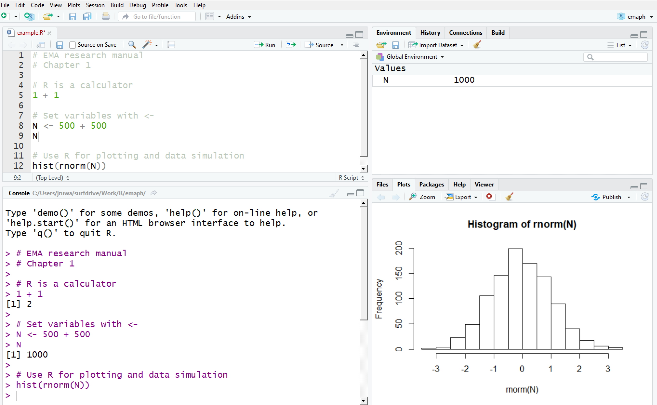
Figure 2.1: The RStudio Interface
Commands are sent to R in the bottom-left pane, named “Console”. To test this, move your cursor to the bottom line, immediately after the prompt sign (>). Next, type the statement below (note that # denotes a comment line; R ignores it, so there is no immediate need to type that). To execute, press Enter.
R will execute the command and return the answer back to the console.
# R is a calculator.
1 + 1
Results of calculations can be saved into variables, by making use of the assignment operator (<-). If you type the name of a variable, R returns its value.
# Use <- to declare and set a variable.
N <- 50 + 50
N
#> [1] 100
To understand why R is such a popular tool for statistical computing, consider the following command, which, in one line, 1) uses the variable N, just created, to 2) generate 100 random numbers from the normal distribution, and 3) plot a histogram of these numbers.
# Plot the histogram of a sample from the normal distribution.
hist(rnorm(N))
The plot appears in the bottom-right pane, as in Figure 2.1.
2.5 Writing R-scripts
Working in the console is a great way to interactively explore R and data, but what if you want to save a particularly useful chain of statements? For this, you can use a script file.
To create a script file, use the RStudio menu: File > New File > R Script. This will open a new tab in the top-left pane of RStudio, where you can edit the script.
In the script window, type all statements that you have been entering in the console in the previous section.
Next, select all lines in the script.
Press
Ctrl+Enterto run the script.
All commands in the script are executed. The commands are echoed in the console pane, and results are shown immediately, as was the case before, when you typed the commands in the console yourself.
Scripts can also be run line by line. Move the cursor to the line you want to run, and press Ctrl+Enter. The line is copied to the console and executed, and the cursor in the script will move to the next line, allowing you to walk through the script, step by step.
2.6 Importing Your Data
Something that confuses new RStudio users, who are more familiar with SPSS, is that it is not obvious how to import data into RStudio. In SPSS, the data are in plain sight. In R, you first have to import the data.
2.6.1 Using RStudio Menus to Import Data
One way to load data into R is to use RStudio’s data import wizard. Follow the steps below to see how this works with data stored in a comma-separated-values (csv) format, a common data format to which many programs, including SPSS and Excel, can export data to.
Download the example csv data file at https://tinyurl.com/yczmjdat (or create a csv-version of one of your own data files).
In RStudio’s menu, choose
File > Import Dataset > From Text (base).In the window that appears, click on
Browseto locate the csv- file on your computer, and clickImportin the next window (see Figure 2.2).
RStudio shows the data, in tabular view, in the top-left window, ready for analysis. You will also find a new entry in the Environment-tab in the top-right pane. When you click the small arrow, at the left of the name, you will see a brief summary of the contents of the data.
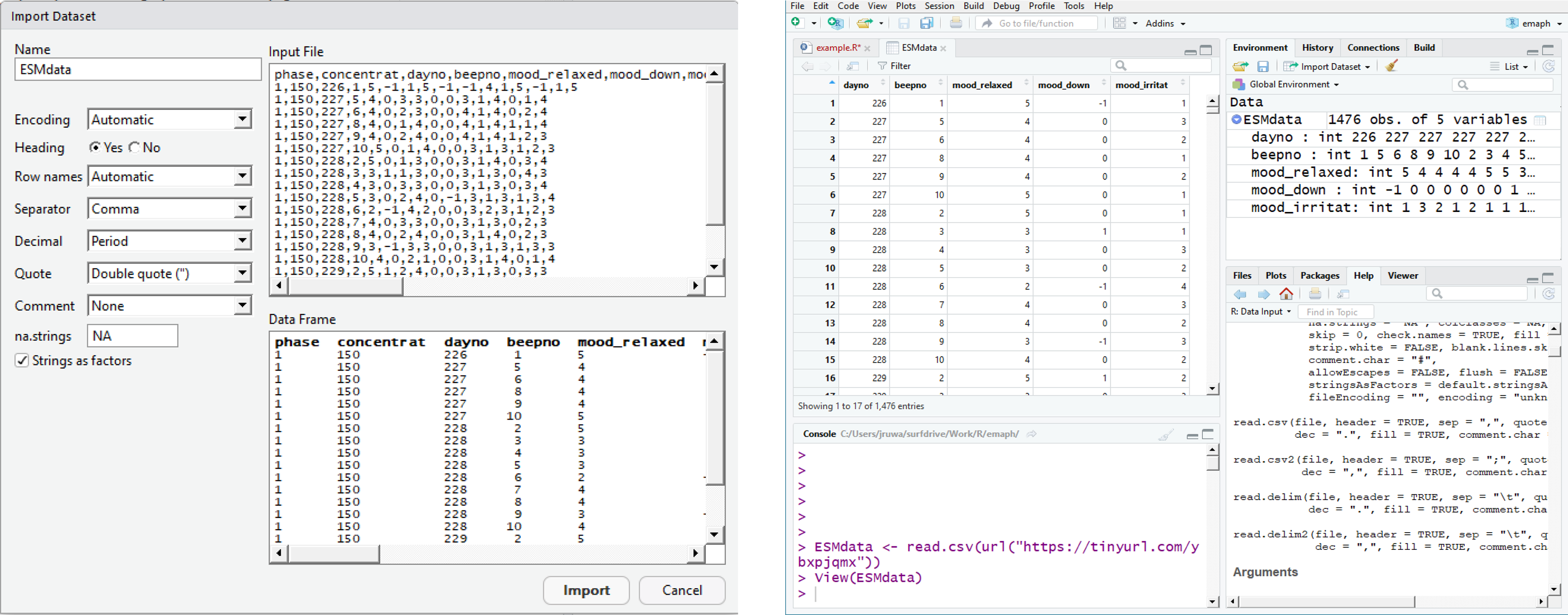
Figure 2.2: RStudio’s CSV import wizard.
2.6.2 Using Functions to Import Data
While RStudio’s Data import wizard is useful, you will probably use it less over time. Most likely, you will convert to using the more efficient R commands to import data. For example, it takes only a single line to download and import the example data.
# Import csv-data, from the internet.
ESMdata <- read.csv(url("https://tinyurl.com/yczmjdat"), row.names = NULL)
2.6.3 Accessing your Data
Since the data is now in the environment (under the name ESMdata), you can use it in other R commands. For example, to produce a more detailed summary of the first four columns of ESMdata, you type:
# Summarize data.
summary(ESMdata)
     dayno           beepno       mood_relaxed     mood_down
 Min.   :  1.0   Min.   : 1.00   Min.   :1.000   Min.   :-3.0000
 1st Qu.: 61.0   1st Qu.: 3.00   1st Qu.:4.000   1st Qu.: 0.0000
 Median :252.0   Median : 5.00   Median :4.000   Median : 0.0000
 Mean   :198.9   Mean   : 5.24   Mean   :4.173   Mean   : 0.1784
 3rd Qu.:303.0   3rd Qu.: 8.00   3rd Qu.:5.000   3rd Qu.: 0.0000
 Max.   :366.0   Max.   :10.00   Max.   :7.000   Max.   : 3.0000
                                                 NA's   :2
  mood_irritat
 Min.   :1.000
 1st Qu.:1.000
 Median :2.000
 Mean   :2.241
 3rd Qu.:3.000
 Max.   :7.000
 NA's   :3
To inspect the first 6 lines of data, type:
# Show first 6 lines of a data frame.
head(ESMdata)
#>   dayno beepno mood_relaxed mood_down mood_irritat
#> 1   226      1            5        -1            1
#> 2   227      5            4         0            3
#> 3   227      6            4         0            2
#> 4   227      8            4         0            1
#> 5   227      9            4         0            2
#> 6   227     10            5         0            1
To view all rows of data in a spreadsheet (as in Figure 2.2), type:
# Show data as spreadsheet.
View(ESMdata)
To work with a specific variable in the data set, use $, for instance, to print the first 20 numbers in the mood_relaxed variable, type:
# Access a single variable in a data frame.
head(ESMdata$mood_relaxed, n = 20)
This allows you to apply functions to specific variables. For example, to calculate the mean of scores in mood_relaxed, type:
# Calculate the mean of a variable.
mean(ESMdata$mood_relaxed)
#> [1] 4.173442
There are many ways in which you can summarize and manipulate your data. At this point, the important milestone is that you have imported and accessed data in R.
2.7 Extending R with Packages
R’s attractiveness lies in the ease with which it can be extended with new functionality. Through so-called packages, which can be freely downloaded from the internet, specialized functions can be added to your work-space.
2.7.1 Installing R-packages from CRAN
Packages can be found at the CRAN website. To browse through the impressive list of available packages, see https://cran.r-project.org/web/packages/available_packages_by_name.html
If you find a package you like, you can install it via the RStudio menu system, choosing Tools > packages. But you can also use the console, via the install.packages function.
A popular package, tidyverse, is used extensively in the examples of this manual. This package comprises a set of popular packages from the creators of RStudio, that greatly simplify working with R. So, while you are at it, install this package now.
# Install a package from CRAN.
install.packages(tidyverse)
The tidyverse contains a package called haven, which allows you to read and write SPSS data files (.sav files). This is very convenient. You don’t have to convert all your SPSS data to csv files. See ?read_spss to learn how to import an SPSS-file (or use the data import wizard, by choosing File > Import Dataset > From SPSS, in RStudio’s top-right pane).
2.7.2 Installing R-packages from GitHub
Not all packages are at CRAN. Many ‘unofficial’ packages are shared at a site called ‘GitHub’. This book’s companion R package emaph, for example, which contains specialized EMA functions data sets, is on GitHub. You need package emaph to run many examples in the book, so let’s install this package now.
GitHub packages can be installed via the install_github function, which is defined in a package called ‘devtools’. So, to install emaph, enter the following in the console:
# Install the GitHub 'emaph' package.
install.packages("devtools")
devtools::install_github("jruwaard/emaph")
2.7.3 Using Packages
To use packages, you have to tell R to load them, each session you want to work with them. You do this with the library function. For example, to use package tidyverse and emaph, type:
# Load packages.
library(tidyverse)
library(emaph)
Once loaded, you can use the functions and data sets of the packages. Package emaph provides data set csd, which contains the data from the ‘critical slowing down’-study (Kossakowski, Groot, Haslbeck, Borsboom, & Wichers, 2017; Wichers, Groot, Psychosystems, ESM, & EWS, 2016), in which a patient recorded his mood, for 239 days (see also Chapter 9).
To plot the irritation levels of this patient in the first six days, using the ggplot function from package ggplot2 (which is in tidyverse), type:
# Using ggplot to plot EMA time series.
ggplot(data = subset(csd, dayno <= 6),
       mapping =  aes(x = beepno, y = mood_irritat)) +
  geom_point() +  geom_step() +
  ylab("Irritation level") +
  scale_x_continuous(breaks = 1:10) +
  facet_wrap(~ dayno, nrow = 2)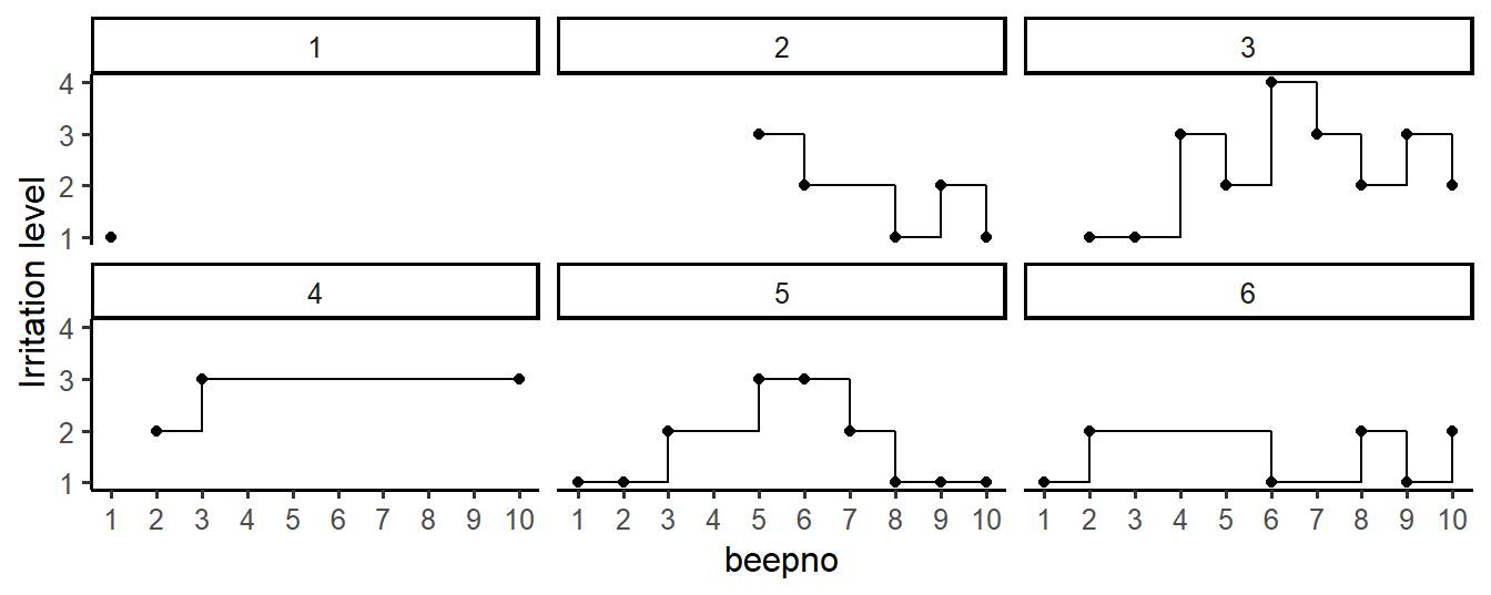
Figure 2.3: Irritation levels of a single patient, in the first six days of an EMA study. Missing values were most prominent at day 1, and irritation varied most at day 3.
2.8 Getting Help
R has no point-and-click menu’s that you can browse through to select a statistical procedure. This is a problem for many new users. What if you want, for example, to generate random numbers from a distribution with a mean of 2 and standard deviation of 4? How to tell this to R?
2.8.1 Using ‘?’ to Consult the Documentation
The good thing is that you already know the name of the function to use, since we used it in the previous section: it is rnorm. To check the documentation of this function, type ?rnorm in the console.
# Use '?' to find the documentation of a function.
?rnorm
This opens the documentation of the rnorm function in the Help-tab, in the bottom right pane, from which you learn that that the rnorm function accepts mean and sd (standard deviation) as additional parameters, which are 0 and 1 default, respectively (which explains why rnorm(100) worked in the previous examples). So, to generate the required numbers, you type:
# Plot the histogram of a custom random sample.
hist(rnorm(1000, mean = 2, sd = 4))
All functions in R are documented, and this documentation is shown in RStudio’s Help pane when you prepend ? to the name of the function in the console.
2.8.2 Using RStudio’s Global Documentation Index Search
What if you do not know the name of a function? Suppose you want to run a t-test for independent groups. Does R have a function for that?
At the top-right of the Help pane, RStudio has a search input field, which allows you to search through all documentation that is installed on your computer. The search field auto-completes your input. If you type a ‘t’ in this field, you will be presented with a list of functions starting with a ‘t’. In this list, you find a likely candidate: a function called t.test. From the documentation of this function (?t.test), you learn that, indeed, this is the function you were looking for.
# Run a t-test, on two simulated samples.

# generate two samples (N = 100 per group) from the normal distribution
A <- rnorm(100); B <- rnorm(100)

# the t-test should be non-significant
t.test(A, B)
#>
#>  Welch Two Sample t-test
#>
#> data:  A and B
#> t = 1.4659, df = 195.6, p-value = 0.1443
#> alternative hypothesis: true difference in means is not equal to 0
#> 95 percent confidence interval:
#>  -0.07314562  0.49672624
#> sample estimates:
#>  mean of x  mean of y
#>  0.0312725 -0.1805178
2.8.3 Learning from Examples
This book contains many R code snippets. By studying these examples, you will become more familiar with R.
Some examples will introduce R language constructs and functions that are unknown to you. Learn from these examples, by using ? on each element that you do not understand.
2.8.4 Google
With Google, you will find many answers to your R questions. Googling for “t-test R”, for example, results in a rich set of online resources. Good resources are:
RSeek (see http://rseek.org/)
Stackoverflow: (see https://stackoverflow.com/questions/tagged/r)
SearchR (see: http://search.r-project.org/)
2.8.5 Read Books
This book does not provide a comprehensive tutorial. There is no need for that, since excellent resources are readily available. A selection is presented below.
Many mental health researchers own a copy of Andy Field’s popular book “Discovering Statistics Using IBM SPSS Statistics” (A. Field, 2013). For those, Field’s R-version of this book, “Discovering Statistics Using R” (A. Field, Miles, & Field, 2012) provides a familiar companion in making the transition to R. See https://www.discoveringstatistics.com/
Free manuals can be found at the official CRAN site. The manuals are dry, but complete and authoritative, since the authors are members of the R core development team. See https://cran.r-project.org/manuals.html (or type
help.start()in the console).While at CRAN, be sure to browse the ‘contributed documentation’-section. On this page, you will find many freely available manuals contributed by the R community. See https://cran.r-project.org/other-docs.html
2.8.6 Online Courses
DataCamp, an online data science education platform, offers several interactive courses in R. See http://www.datacamp.com
The Try-R course at the CodeSchool website provides an alternative to DataCamp. See: http://tryr.codeschool.com/
The Quick-R website provides a concise introduction to R. See https://www.statmethods.net/
2.8.7 Learn R, in R
Package swirl contains a set of interactive courses that teach many aspects of the R language. See http://swirlstats.com
# Start the interactive swirl-course.
install.packages("swirl")
library("swirl")
swirl()
References
Kossakowski, J. J., Groot, P. C., Haslbeck, J. M. B., Borsboom, D., & Wichers, M. (2017). Data from ‘critical slowing down as a personalized early warning signal for depression’. Journal of Open Psychology Data, 5(1). https://doi.org/10.5334/jopd.29
Wichers, M., Groot, P. C., Psychosystems, ESM, & EWS. (2016). Critical slowing down as a personalized early warning signal for depression. Psychotherapy and Psychosomatics, 85(2), 114–116. https://doi.org/10.1159/000441458
Field, A. (2013). Discovering statistics using IBM SPSS statistics (4th ed.). Sage Publications Ltd.
Field, A., Miles, J., & Field, Z. (2012). Discovering Statistics Using R (1st ed.). Paperback; SAGE Publications Ltd.