Chapter 9 Early Warning Signs of Depression
One of the promises of EMA is that it might detect signs of mental health deterioration in an early stage. Subtle changes in time series of mood variables, for example, might signal a depression relapse. If we can detect these changes, preventive interventions can be triggered to avoid the relapse.
But what changes, exactly, should we look for? What are these early warning signs?
9.1 Critical Slowing Down
Critical Slowing Down (CSD) is a concept from dynamic systems theory. In dynamic systems, state transitions are preceded by a change in which the system reacts to disturbances. In a stable state, the system quickly recovers from disturbances. Prior to a transition to a new state, however, the system takes more and more time to recover back to its current state: the variance and auto-correlation of the system increases (Dakos et al., 2008; Scheffer et al., 2009).
In this chapter, we re-analyze data from a study that aimed to demonstrate CSD in EMA-data of a single patient with a history of major depression (Groot, 2010, Kossakowski et al. (2017); Wichers et al., 2016). The patient, a 57-year old male, used EMA to monitor himself during a 239-day single-case double-blind medication reduction trial. During the experiment, he experienced a relapse, and Wichers and colleagues showed how variance and auto-correlation in the EMA data increased, several weeks prior to this relapse. The transition appeared to be preceded by CSD.
We will try to reconstruct the finding, using an alternative analysis strategy. One of the limitations of the Wichers et al analysis is that auto-correlation was analyzed at lag 1 only (i.e., only the correlation between t and t-1 was considered). With another analysis technique, called ‘Detrended Fluctuation Analysis’, all lags can be considered.
To conduct the analysis, we need three R packages:
Raw EMA data of this study were published in the public domain (Kossakowski et al., 2017). We included the data in the
emaphpackage.To manipulate the raw data and reconstruct the plots of the article, we are going to use several functions from
tidyversepackages.DFA is implemented in package
nonlinearTseries, so we will need that as well.
# Required libraries for the CSD-study re-analysis.
library(emaph)
library(tidyverse)
library(nonlinearTseries)
9.2 Plotting the Course of Depression
Let’s take a look at the development of the depressive symptoms of the patient first. These were tapped with weekly assessments of the depression scale of the ‘Symptom Checklist-90-Revised’ (SCL-90-R; Derogatis, 1994), a well-established self-report questionnaire.
The code below reconstructs Figure 1 of the Wichers et al article. It plots the SCL90-R depression scale score over the time. Around day 120, the depression score increased considerable: the patient experienced a relapse.
# Plot depression score.
dep <- csd %>% select(dayno, scl90r_dep) %>%
  filter(!is.na(scl90r_dep)) %>% unique

# plot dep + change point (day 120 in our data)
ggplot(dep, aes(x = dayno, y = scl90r_dep, group = 1)) +
  geom_step() +
  xlab("Days") + ylab("SCL-90-R Depression") +
  theme_classic()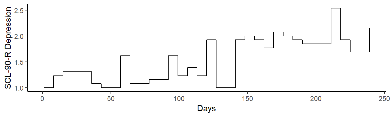
Figure 9.1: SCL-90 depression score, over the study period
9.3 Mental state EMA Items
Wichers and colleagues selected 13 items from the full EMA data set, which they grouped in 5 factors: positive affect (pa; 4 items), negative affect (na; 4 items), mental unrest (mu; 3 items), suspiciousness (su; 1 item), and worrying (wo; 1 item). From these factors, an overall mental state sum score can be calculated.
# Mood states calculation.

# positive affect
pa_items <- c("mood_enthus", "mood_cheerf",
              "mood_strong", "mood_satisfi")

csd$pa <- csd %>%
  select(pa_items) %>%
  rowMeans(., na.rm = TRUE)
csd$pa <- -csd$pa

# negative affect
na_items <- c("mood_lonely", "mood_anxious",
              "mood_guilty", "mood_doubt")

csd$na <- csd %>%
  select(na_items) %>%
  rowMeans(., na.rm = TRUE)

# mental unrest
mu_items <- c("mood_irritat", "pat_restl",
              "pat_agitate")
csd$mu <- csd %>%
  select(mu_items) %>%
  rowMeans(., na.rm = TRUE)

# 'single-item' states
csd$su <- csd$mood_suspic
csd$wo <- csd$pat_worry

# global mental state score
csd$ms <- rowSums(csd[c("pa", "na", "mu", "su", "wo")])
Rows, in which one or more of the factors have missing values, are removed from the analysis. In a full analysis, options to impute the missing values could and should be considered. However, since only 3 of the 1476 rows have missing item scores, not much is probably lost by running a simple complete-case analysis.
# Missing values removal.

# count number of items with missing items, per row
csd$nna <- csd %>%
  select(matches("mood_")) %>%
  is.na(.) %>% rowSums

# drop rows with missing values
csd <- csd %>% filter(nna == 0)
9.4 Running the DFA
We are now ready to run the DFA analysis. We split the full series in 31-day overlapping windows, in steps of 1 day (i.e., day 1-31, day 2-32, etc.), calculate the DFA of each window and save that value so that we can compare it to the weekly depression assessments.
# Running the DFA.

# prepare result rows: one row for each day
d <- NULL
d <- csd %>%
  group_by(dayno) %>%
  summarise(ms = mean(ms))
d$ms_dfa = NA

# determine DFA, in a moving window of 31 days
window <- 31
for (i in seq(window, max(csd$dayno), 1)) {

  # get the sliding window data
  w <- subset(csd, dayno > (i - window) & dayno <= i)

  # dfa: ms
  dfa.analysis <- dfa(time.series = w$ms,
                      npoints = 30,
                      window.size.range = c(10, nrow(w)),
                      do.plot = FALSE)

  fgn.estimation <- estimate(dfa.analysis,
                            do.plot = FALSE,
                            fit.col = "blue", fit.lwd = 2, fit.lty = 2,
                            main = "Fitting DFA to fGn")

  d$ms_dfa[d$dayno == i] <- fgn.estimation
}
9.5 Results
We can now plot the DFA indicator over time, to see whether it peaks prior to the onset of the relapse. As can be seen, the DFA-indicator clearly peaks prior to the onset of the relapse, around day 110 (where the color changes to red). Interestingly, a second peak is reached at the end of the experiment, around day 239, indicating - perhaps - a recovery from the relapse.
# Plot DFA results.
ggplot(na.omit(d),
      aes(x = dayno, y = ms_dfa,
          colour = factor(dayno < 120),
          group = 1)) +
  geom_point() +
  geom_line() +
  ylab("dfa (31-day window)") +
  xlim(c(0, 250)) +
  guides(color = FALSE) +
  theme_classic()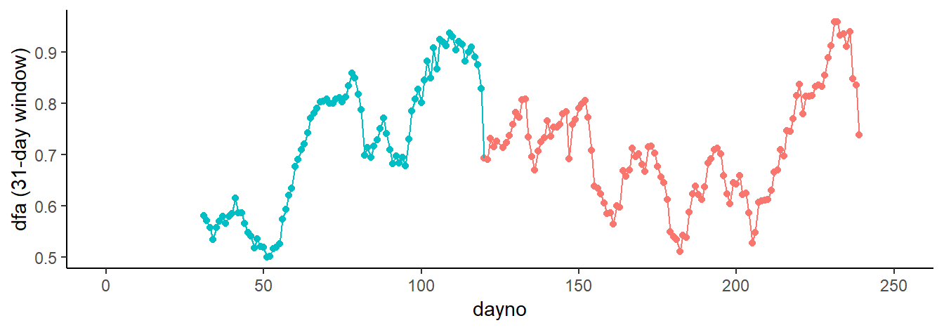
Figure 9.2: Results of the DFA analysis.
9.6 Discussion
Our re-analysis replicates the main finding of the Wichers et al article ((Wichers et al., 2016)): several weeks prior to a depression relapse, as predicted by complex systems theory, the variance and auto-correlation in EMA mood ratings increased.
Potential clinical applications, of course, are clear. If clinically relevant changes can be predicted algorithmically from EMA ratings, automated patient feedback systems could help to prevent pending deterioration or consolidate the path towards recovery.
One swallow, however, does not make summer. Yes, in this case, the DFA-indicator peaked prior to the relapse. This could be a mere coincidence. The predictive power of CSD needs to be confirmed in larger samples and prospective studies. Given the theoretical background, successful applications of CSD in other domains, and the present finding, the spending of resources on such studies seems warranted.
Important additional questions remain to be answered. When it predicts a state change, what is the expected delay between this prediction and the change? Does a critical DFA-value exist? Given that critical value, are false positive and false negative rates of this prediction acceptable? These are important questions that should be answered before any clinical application of DFA can be considered.
Re-analysis of data from completed clinical studies, in which EMA data were collected, may be a first step to further explore the value of CSD. One option, for example, would be to re-analyze data from the E-COMPARED study (Kleiboer et al., 2016). In this trial, patients, who were treated for major depression, completed weekly self-report questionnaires (the Patient Health Questionnaire; PHQ-8, Kroenke et al., 2009) and daily EMA mood ratings throughout treatment, which lasted up to 16-week. Since CSD is an indicator of any state change (i.e., irrespective of whether the change is clinically “good” or “bad”), theory would predict a (lagged) relationship between CSD (i.e., the DFA-score) and clinically significant changes in PHQ-scores (Jacobson & Truax, 1991).
References
Dakos, V., Scheffer, M., Van Nes, E. H., Brovkin, V., Petoukhov, V., & Held, H. (2008). Slowing down as an early warning signal for abrupt climate change. TL - 105. Proceedings of the National Academy of Sciences of the United States of America, 105 VN -(38), 14308–14312. https://doi.org/10.1073/pnas.0802430105
Scheffer, M., Bascompte, J., Brock, W. A., Brovkin, V., Carpenter, S. R., Dakos, V., … Sugihara, G. (2009). Early-warning signals for critical transitions. https://doi.org/10.1038/nature08227
Groot, P. C. (2010). Patients can diagnose too: How continuous self-assessment aids diagnosis of, and recovery from, depression. Journal of Mental Health, 19(4), 352–362. https://doi.org/10.3109/09638237.2010.494188
Kossakowski, J. J., Groot, P. C., Haslbeck, J. M. B., Borsboom, D., & Wichers, M. (2017). Data from ‘critical slowing down as a personalized early warning signal for depression’. Journal of Open Psychology Data, 5(1). https://doi.org/10.5334/jopd.29
Wichers, M., Groot, P. C., Psychosystems, ESM, & EWS. (2016). Critical slowing down as a personalized early warning signal for depression. Psychotherapy and Psychosomatics, 85(2), 114–116. https://doi.org/10.1159/000441458
Derogatis, L. R. (1994). Symptom Checklist-90-R (SCL-90-R): Administration, scoring, and procedures manual. Minneapolis, MN: NCS Pearson.
Kleiboer, A., Smit, J., Bosmans, J., Ruwaard, J., Andersson, G., Topooco, N., … Riper, H. (2016). European COMPARative Effectiveness research on blended Depression treatment versus treatment-as-usual (E-COMPARED): Study protocol for a randomized controlled, non-inferiority trial in eight European countries. Trials, 17(1). https://doi.org/10.1186/s13063-016-1511-1
Kroenke, K., Strine, T. W., Spitzer, R. L., Williams, J. B., Berry, J. T., & Mokdad, A. H. (2009). The PHQ-8 as a measure of current depression in the general population. Journal of Affective Disorders, 114(1-3), 163–173. https://doi.org/10.1016/j.jad.2008.06.026
Jacobson, N. S., & Truax, P. (1991). Clinical significance: A statistical approach to defining meaningful change in psychotherapy research. Journal of Consulting and Clinical Psychology, 59(1), 12–19. https://doi.org/10.1037/0022-006X.59.1.12