Chapter 6 Activity
The objective study of human physical activity is one of the exciting opportunities created by passive EMA (Marszalek et al., 2014). Through technological advances in mobile sensing, we are now able to continuously monitor (in-)activity of participants in every-day life, with little to no participant burden.
While questions remain with regard to the validity, reliability and clinical utility of passive EMA of specific activities, such as (disturbed) sleep, sedentary behavior, and energy expenditure (see, e.g., Feehan et al., 2018; Gomersall, Ng, Burton, Pavey, & Gilson, 2016), an increasing number of mental health studies are including activity tracking devices to better understand sleep habits, circadian rhythm disorders and depression (see, e.g., Cornet & Holden, 2018; Saeb et al., 2015; Saunders et al., 2016; Tahmasian, Khazaie, Golshani, & Avis, 2013).
In this chapter, we will discuss two passive EMA methods to assess physical activity: actigraphy and geotracking. Of these two, actigraphy has been used most in human clinical research. However, due to the massive adoption of smartphones, researchers increasingly collect geolocation data as well, inspired perhaps by the elaborate geolocation data analysis techniques that have been developed in the past decades in wildlife telemetry research (Tomkiewicz, Fuller, Kie, & Bates, 2010).
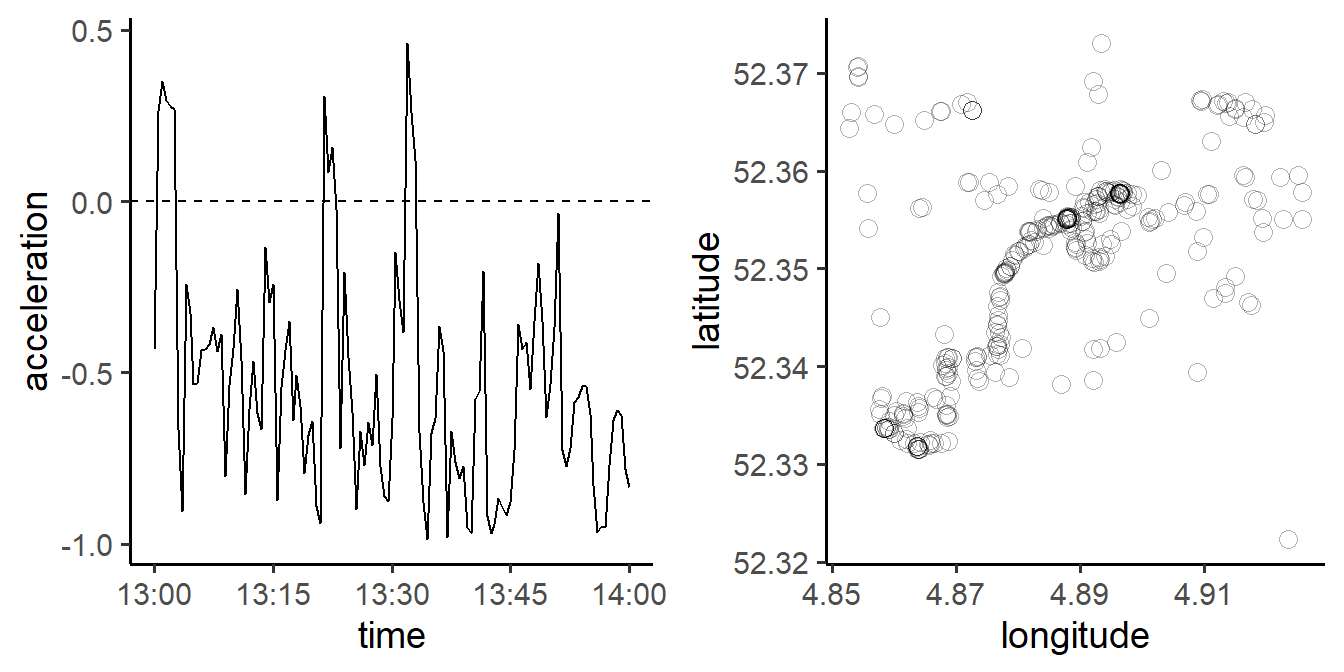
Figure 6.1: Actigraphy (left) and Geotracking (right): two methods for passive ecological momentary assessment of activity.
6.1 Actigraphy
Accelerometers are micro electro-mechanical systems (MEMS) that measure changes in acceleration forces (i.e., both static forces - earth’s gravity - and dynamic forces - caused by movement), typically simultaneously on the vertical (Y), horizontal right-left (X) and horizontal front-back axis (Z). Through actigraphy, we study the frequency, duration, and intensity of physical activity. Figure 6.2 shows one hour of data collected from a wrist-worn GENEActiv accelerometer. As can be seen, three accelerometers (X, Y, Z) were simultaneously providing data. Data were sampled with a frequency of 30 Hertz (Hz; thirty measurements per second - which is common), but sub-sampled here to 0.1Hz (one measurement every 10 seconds), for practical reasons. If we would have plotted the data at 30Hz, the plot would have included 108.000 data points. At 0.1Hz, this reduces to 360 points.
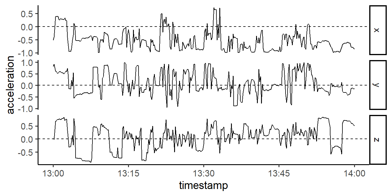
Figure 6.2: One hour of raw data collected with a wrist-worn GENEActiv accelerometer, sub-sampled to 10-second epochs (0.1 Hz)
Data shown are included in package emaph, and the R-code to reproduce the plot is listed below. Use this to familiarize yourself with actigraphy data. If you want to see how sub-sampling affects the number of points to plot, for example, you can set different values in the round_date function. For example, to get a point for each five seconds (0.2Hz), you would set the argument of this function to 5 seconds.
# Plot one hour of emaph accelerometer data (of person 1).
library(dplyr)
library(ggplot2)
d <-  subset(emaph::geneactiv, timestamp > "2018-06-01 13:00" &
                           timestamp < "2018-06-01 14:00" &
                           id == 1)
d$timestamp <- lubridate::round_date(d$timestamp, "10 seconds")
d <- d %>% group_by(timestamp) %>% summarise_all(.funs = mean) %>%
  tidyr::gather(key = "sensor", value = "value", x, y, z)

ggplot(d, aes(timestamp, value)) + geom_line() +
  geom_hline(yintercept = 0, linetype = 2) + facet_grid(rows = vars(sensor) , scales = "free_y")
6.1.1 Data cleaning
Raw accelerometer data need to be cleaned before analyses can be run. Typical data import work-flows include re-calibration (to reduce systematic measurement error; Van Hees et al., 2014), the detection of non-wear periods (to ensure that non-informative data are removed or imputed), sub-sampling (reducing the sample rate to reduce analysis time) and filtering/aggregation (to smoothen the signal and reduce the impact of outliers, measurement error and occasional missing values). Study results can be highly dependent on these initial steps, which, unfortunately, are also complex and time-consuming. Specialized R-packages exist to help you with this (see, for example, package GGIR and GENEAread, which are described in more detail in Chapter 12).
6.1.2 Feature Extraction
Properties of the signals that are of interest are highly dependent on the focus of the study. Highly detailed analysis of local peaks in the signal might be needed, for instance to reveal an association between activity and reported events. But analyses can also be more global, for instance when accelerometer data are used to study circadian rhythms in activity. Several approaches exist to combine the X, Y, Z measurements into a single meaningful metric. Two popular metrics are the ‘Signal Vector Magnitude’ (SVM) and the ‘Euclidean Norm Minus One’ (ENMO). Validation studies suggest that ENMO should be the preferred metric (Van Hees et al., 2014, 2015), although recent findings also suggest that alternative metrics should perhaps be considered when sedentary and light activities are of interest (Bai et al., 2016).
SVM and ENMO are closely related. SVM is the magnitude of the raw tri-axial signals (the Euclidean distance in the three-dimensional space), i.e. SVM = sqrt(x^2 + y^2 + z^2). ENMO is the corrected SVM: the vector magnitude remaining after removing one Earth Standard Gravitational unit (1g = 9.81 m/s^2), with negative values rounded to 0, i.e. ENMO = max(SVM - 1, 0). The metrics can, in principle, be calculated for each {x, y, z}-data point in the raw series. Typically, however, the metrics are calculated for time-windows (called epochs), in which case the mean can be used to characterize the overall activity in each epoch.
Figure 6.3 shows the development of ENMO over one day, as sampled by GENEActiv accelerometers that were worn by a young adult (top) and a middle-aged person (bottom). This figure is much easier to interpret than the plot of the raw x-y-z values in Figure 6.2. Activity levels over the day follow a similar pattern, but the activity levels in the two plots are strikingly different. Age appears to matter here: activity levels of the middle-aged person are consistently lower than those of the young adult.
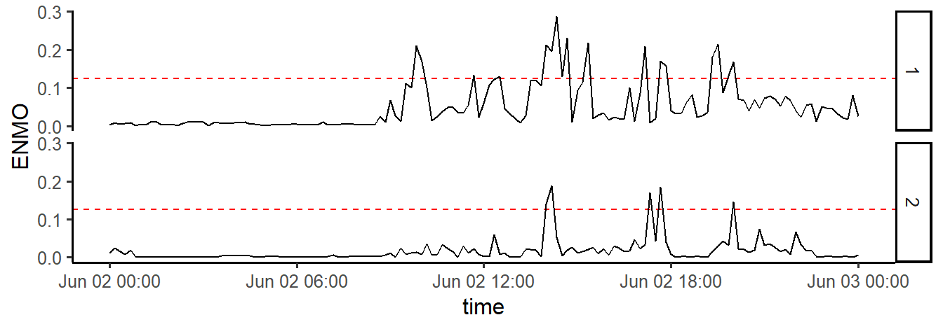
Figure 6.3: One day of data of the two persons in the GENEA data set of package ‘emaph’, summarised with ENMO, in 10-minute epochs
For SVM and ENMO, cut-off values for various activity classes have been determined (Da silva et al., 2014; Hildebrand, Van Hees, Hansen, & Ekelund, 2014; Kim et al., 2017; Rowlands, Yates, Davies, Khunti, & Edwardson, 2016). Although these cut-offs vary somewhat from study to study, a suggested pragmatic ENMO cut-off for Moderate-to-Vigorous-Physical-Activity (MVPA) is 0.125g (125 milligravity units; Femke Lamers, personal communication, 15 november 2018). The dotted line in Figure 6.3 marks this cut-off.
With this cut-off, we can summarize the two series shown in Figure 6.3 by the number of times on which ENMO is higher than the MVPA cut-off. The daily MVPA-count for the young adult is 17. For the middle-aged person, this is 5: considerably lower.
You should be aware that the choice of the width of the epoch matters when MVPA-counts are calculated. By averaging values in each window, ENMO acts as a smoother, which may prevent you from the detection of short bursts of activity when the window is large. If we would have used a 5-second window to generate Figure 6.3, for example, the MVPA-counts would go up considerably for each person.
6.2 Geotracking
6.2.1 The Geographic Coordinate System
In the geographic coordinate system, each location on the earth is uniquely represented by two numbers: Latitude and Longitude. Latitude marks the north–south position of a point on the earth’s surface, and longitude marks the east-west position (see Figure 6.4). The center of Amsterdam, for example, is {latitude: 52.37022; longitude: 4.89517}, which can be verified by punching these numbers in Google maps.
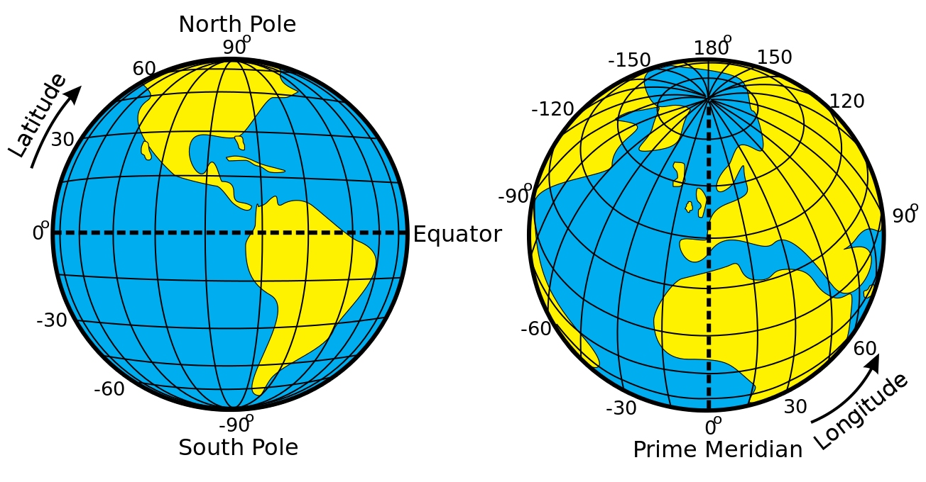
Figure 6.4: Latitude and Longtitude of the Earth (source: WikiPedia).
6.2.2 The Global Positioning System
The Global Positioning System (GPS) is a satellite-based radio-navigation system that provides geolocation and time information. With GPS-receivers, latitude and longitude can be determined, to track geographical locations and movement. Due to the increasing ease with which GPS-data can be collected via modern smartphones, recent years have witnessed a marked increase in the use of GPS-based activity measures in the study of mental health.
Figure 6.5 shows GPS-data of two people, collected over a period of four weeks, via the Google timeline smartphone app. Data can be found in the emaph package (see ?locations).
# Plot four-week location history of emaph location data
library(ggplot2)
library(emaph)

d <- subset(locations,
            accuracy <= 50 &
              lon >=  4.80 & lon <=  5.00 &
              lat >= 52.25 & lat <= 52.50) %>%
  sample_n(4000)

ggplot(d, aes(lon, lat)) +
  geom_point(alpha = .2,  shape = 21, size = 3) +
  xlab("longitude") + ylab("latitude") +
  facet_wrap(~ id)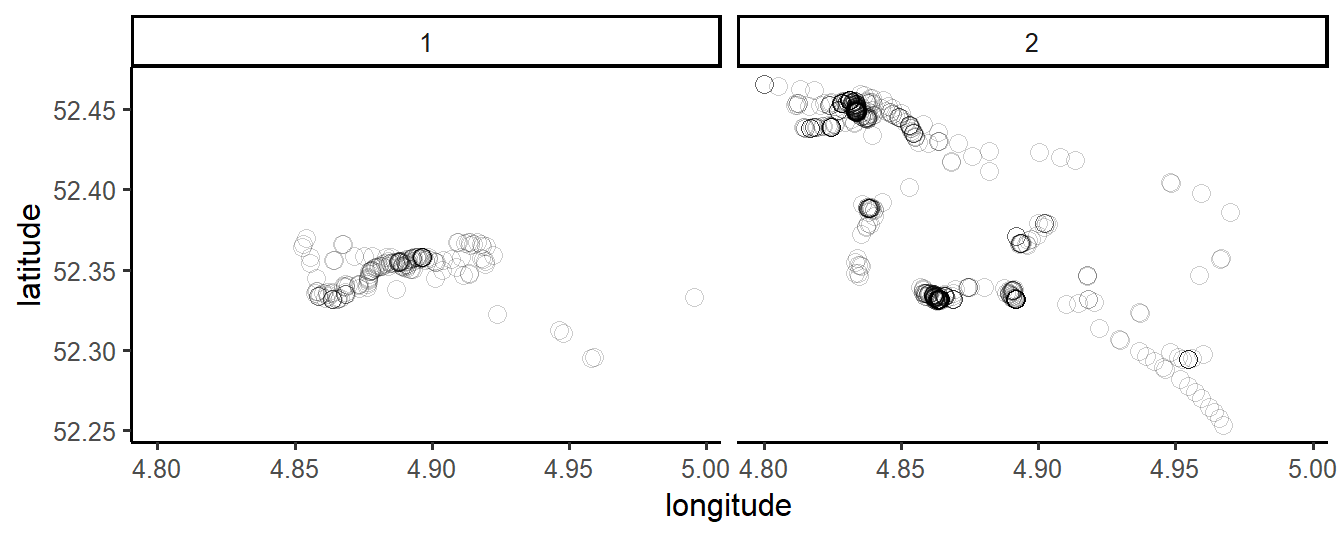
Figure 6.5: Four-week location history of two people, collected with Google Timeline.
Data-points are superposed, using transparent colors, to make a distinction between locations that were visited once (light areas) and places that were visited many times (darker areas). From the plot, we learn that these two people both lived and worked in the Amsterdam area (latitude and longitude are close to the coordinates of Amsterdam center). We also see that they shared a frequently visited location (they were co-workers, working in the same building). Locations of person 1 reveal that this person’s home was probably in Amsterdam, while the locations of person 2 show that this person’s home was probably located in an Amsterdam suburb. Commuting patterns (i.e., the recurrent traveling between the place of residence and place of work) are clearly visible.
It should be noted, though, that person 1 contributed much less data (n = 722) than person 2 (n = 14031). This can be explained by the different devices that were used by both: Person 1 used an iPhone (with standard GPS-settings) and Person 2 used a Sony Z1 Android (with high-precision GPS features enabled). This device-related variability in GPS sample rates and accuracy is one of the primary challenges of naturalistic EMA research and EMI applications.
The problem with the (in)accuracy of GPS-data is further illustrated by Figure 6.6, in which all data points are plotted that were registered by the smartphone of person 2 between 02:00 and 06:00, At those hours, the person was sleeping, in the bedroom of his house. He did not move. Yet, if we would take the GPS-data for granted, he regularly took a nightly random walk in the park. The red dot in the figure marks the median coordinate. This coordinate is very accurate: it marks the bedroom. All individual data points, however, fail to identify this location.
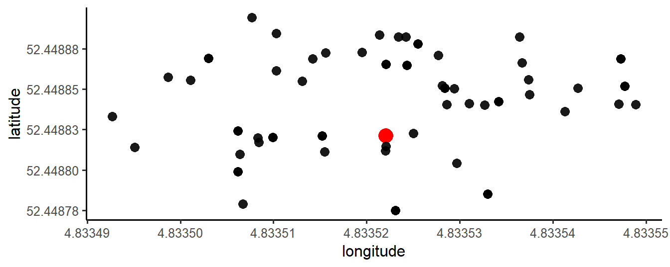
Figure 6.6: Nightly GPS-fluctuations, revealing inaccurate location measurements
6.2.3 GPS-based Activity Measures
Raw GPS-data reflect series of locations rather than activity per se. However, measures of activity can be extracted from these data.
Table 6.1 shows some of the measures that were derived from GPS data in a small (n = 28) study exploring the correlation between passive EMA data and depression, conducted by researchers of Northwestern University (Saeb et al., 2015). The researchers calculated total distance, location variance, the number of places visited by the participants during the study [using the K-means clustering algorithm, Hartigan & Wong (1979), which is implemented in R as kmeans), the percentage of time spent at home (defined as a top 3 place which was most frequently visited between 24:00 and 6:00), and circadian movement - the consistency of location visits based on a 24-hour period. Circadian movement and location variance were found to be correlated with PHQ-9 scores in this study, but not - however - in a follow-up study, which included more participants (Saeb, Lattie, Kording, & Mohr, 2017).
| Name | Formula |
|---|---|
| Total distance between locations | \(\sum(distance((lat_{t}, lon_{t}), (lat_{t-1}, lon_{t-1})\) |
| Location variance | \(log(\sigma_{lon}^2 + \sigma_{lat}^2)\) |
| N Places | kmeans(loc, lat) |
| Home Stay | time(cluster[home]) / time(clusters[j]) |
| Circadian Movement | \(\sum(psd(f_i) / (i1 - i2)\) |
References
Marszalek, J., Morgulec-Adamowicz, N., Rutkowska, I., Kosmol, A., Marszalek, J., Morgulec-Adamowicz, N., … Kosmol, A. (2014). Using ecological momentary assessment to evaluate current physical activity. BioMed Research International, 2014, e915172. https://doi.org/10.1155/2014/915172
Feehan, L. M., Geldman, J., Sayre, E. C., Park, C., Ezzat, A. M., Yoo, J. Y., … Li, L. C. (2018). Accuracy of fitbit devices: Systematic review and narrative syntheses of quantitative data. Journal of Medical Internet Research. https://doi.org/10.2196/10527
Gomersall, S. R., Ng, N., Burton, N. W., Pavey, T. G., & Gilson. (2016). Estimating physical activity and sedentary behavior in a free-living context: A pragmatic comparison of consumer-based activity trackers and actigraph accelerometry. Journal of Medical Internet Research. https://doi.org/10.2196/jmir.5531
Cornet, V. P., & Holden, R. J. (2018). Systematic review of smartphone-based passive sensing for health and wellbeing. Journal of Biomedical Informatics, 17(1), 120–132. https://doi.org/10.1016/j.jbi.2017.12.008
Saeb, S., Zhang, M., Karr, C. J., Schueller, S. M., Corden, M. E., Kording, K. P., & Mohr, D. C. (2015). Mobile phone sensor correlates of depressive symptom severity in daily-life behavior: An exploratory study. Journal of Medical Internet Research, 17(7). https://doi.org/10.2196/jmir.4273
Saunders, K., Palmius, N., Vos, M. de, Bilderbeck, A., Geddes, J., & Goodwin, G. (2016). Depression detection in bipolar disorder using geolocation data. Bipolar Disorders. https://doi.org/10.1109/TBME.2016.2611862
Tahmasian, M., Khazaie, H., Golshani, S., & Avis, K. T. (2013). Clinical application of actigraphy in psychotic disorders: A systematic review. Current Psychiatry Reports. https://doi.org/10.1007/s11920-013-0359-2
Tomkiewicz, S. M., Fuller, M. R., Kie, J. G., & Bates, K. K. (2010). Global positioning system and associated technologies in animal behaviour and ecological research. Philosophical Transactions of the Royal Society of London B: Biological Sciences, 365(1550), 2163–2176. https://doi.org/10.1098/rstb.2010.0090
Van Hees, V. T., Fang, Z., Langford, J., Assah, F., Mohammad, A., Silva, I. C. da, … Brage, S. (2014). Autocalibration of accelerometer data for free-living physical activity assessment using local gravity and temperature: An evaluation on four continents. Journal of Applied Physiology, 117(7), 738–744. https://doi.org/10.1152/japplphysiol.00421.2014
Van Hees, V. T., Sabia, S., Anderson, K. N., Denton, S. J., Oliver, J., Catt, M., … Singh-Manoux, A. (2015). A novel, open access method to assess sleep duration using a wrist-worn accelerometer. PLoS One, 10(11). https://doi.org/10.1371/journal.pone.0142533
Bai, J., Di, C., Xiao, L., Evenson, K. R., LaCroix, A. Z., Crainiceanu, C. M., & Buchner, D. M. (2016). An activity index for raw accelerometry data and its comparison with other activity metrics. PLoS ONE. https://doi.org/10.1371/journal.pone.0160644
Da silva, I. C., Van Hees, V. T., Ramires, V. V., Knuth, A. G., Bielemann, R. M., Ekelund, U., … Hallal, P. C. (2014). Physical activity levels in three Brazilian birth cohorts as assessed with raw triaxial wrist accelerometry. International Journal of Epidemiology. https://doi.org/10.1093/ije/dyu203
Hildebrand, M., Van Hees, V. T., Hansen, B. H., & Ekelund, U. (2014). Age group comparability of raw accelerometer output from wrist-and hip-worn monitors. Medicine and Science in Sports and Exercise. https://doi.org/10.1249/MSS.0000000000000289
Kim, Y., White, T., Wijndaele, K., Sharp, S. J., Wareham, N. J., & Brage, S. (2017). Adiposity and grip strength as long-Term predictors of objectively measured physical activity in 93 015 adults: The UK Biobank study. International Journal of Obesity. https://doi.org/10.1038/ijo.2017.122
Rowlands, A. V., Yates, T., Davies, M., Khunti, K., & Edwardson, C. L. (2016). Raw Accelerometer Data Analysis with GGIR R-package: Does Accelerometer Brand Matter? Medicine and Science in Sports and Exercise. https://doi.org/10.1249/MSS.0000000000000978
Hartigan, A., & Wong, M. A. (1979). A K-Means Clustering Algorithm. Journal of the Royal Statistical Society. https://doi.org/10.2307/2346830
Saeb, S., Lattie, E. G., Kording, K. P., & Mohr, D. C. (2017). Mobile Phone Detection of Semantic Location and Its Relationship to Depression and Anxiety. JMIR mHealth and uHealth. https://doi.org/10.2196/mhealth.7297