Chapter 4 Data Management
In a typical EMA study, lots of data are collected. Repeated self-reports, GPS-data, accelerometer data, background demographic data and traditional questionnaire data quickly add up to gigabytes of raw data. Without proper data management, the EMA researcher would drown in these data. Fortunately, R and RStudio are useful aids to prevent this from happening. R is very flexible in the management of multiple data files, and RStudio includes a handy feature, called “Projects”, with which data and analysis scripts can be stored in an orderly fashion.
4.1 Using RStudio-projects
RStudio projects can be opened by double-clicking existing projects, or by creating new projects from RStudio’s file menu. To create a new project, choose File > New Project.... You will be asked to specify the project name and its disk location (as shown in 4.1, after which the project will open in a new window.
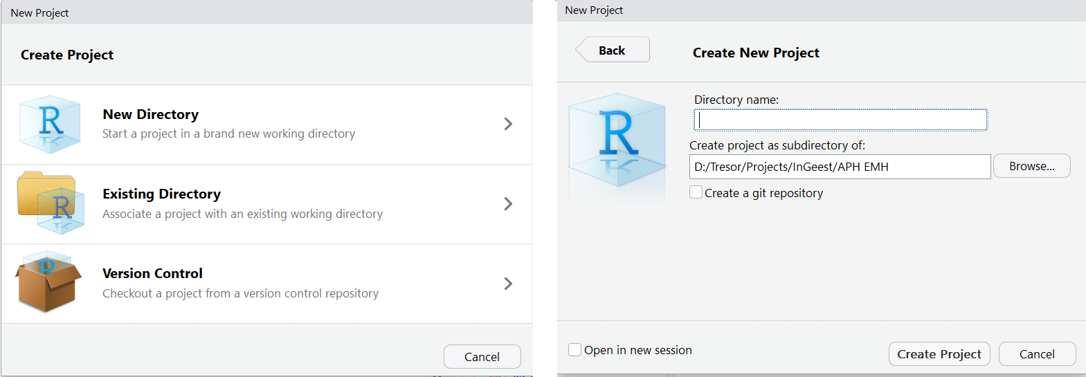
Figure 4.1: creating a project in RStudio
One of the advantages of using RStudio Projects is that projects set the working directory to the project directory location. You can verify this by asking R to print the current working directory, by typing the getwd() function in the console, while the project is open.
This may look like a trivial feature. It is, however, a great advantage, because it allows for the use of relative paths, which is very convenient. For example, to open a data source in a script, you no longer have to specify its full path (e.g., ‘D:/work/projects/my_ema_project/data/raw/ema_data.csv’). With relative paths, you can simply type ‘data/raw/ema_data.csv’. This saves typing, but, more importantly, it allows you to freely move your projects to other locations, without breaking the proper functioning of your scripts.
4.2 An Example Project Directory Structure
RStudio imposes no limitations to the contents of project directories. You are free to organize the project in the way you want. In clinical research, however, you are advised to choose a structure that aids you best to implement the following research guidelines:
You should adhere strictly to a clear and logical directory structure, to ensure that co-workers and external auditors can quickly grasp and reproduce your work;
Raw data should be part of your project, so that results can be traced back to their source;
Cleaned data should be separated from raw data, and data cleaning procedures should be explicit and reproducible;
Data and analyses should be clearly separated;
All analyses should be explicit and reproducible;
Output of (published) analyses should be saved.
A directory structure based on these guidelines is listed in Figure 4.2. It shows the organization of a (hypothetical) project in which data were collected via:
an online survey system, to assess demographics and pre/post study depression severity (with the PHQ-9 questionnaire, Kroenke et al. (2009)),
an active EMA smartphone app, to assess day-to-day changes in mood, and
an accelerometer to assess activity levels.
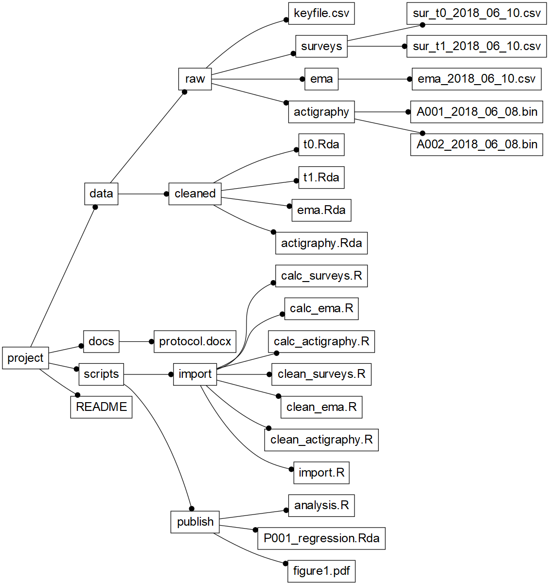
Figure 4.2: Example project directory structure
The full project, including example data and R-scripts, is available for download at https://tinyurl.com/yd7mx32c. Download, unzip, and double-click the ‘APH EMA Project.Rproj’ file, to open the project in RStudio. Note that this is a large download (~134MB), because it contains large accelerometer data files.
4.3 Data
Full reproducibility implies that raw data can be traced back to the source. Wherever possible, this should translate to the availability of raw study data in your project.
In the example project, unprocessed data files exported from the three data collection systems (i.e., survey data, EMA data, and actigraphy data) are stored in the ’data/raw“-directory’, in separate sub-directories per data type.
In ‘data/raw/surveys’, we find two files: 1) ‘sur_t0_2018_06_10.csv’, containing the results of the demographic questionnaire and the PHQ-9 pre-test, and 2) ‘sur_t1_2018_06_10.csv’, containing the results of the PHQ-9 post-test. In exports of such survey systems, data from all participants are typically stored in one file per assessment moment. Note how the export date is added to the files, to make sure that future updates are only used in the analysis when explicitly noted.
In ‘data/raw/ema’, we find one file: ‘ema_2018_06_10.csv’, containing the results of the EMA mood measurements of all participants, exported from the back-office of the EMA platform.
Finally, in ‘data/raw/actigraphy’, we see two ‘.bin’ files: binary data files that were exported from, e.g., GENEActiv smart watches, that were worn by two participants. Unlike the survey and EMA mood data, each data file in this directory contains data of one participant. Actigraphy data are high-volume data: these files are typically large (500MB is no exception). By using the ‘.bin’ format, in which data are compressed, disk space is saved (in uncompressed format, data in a single .bin file can amount up to 2 GB).
In ‘data/raw’, a final very important file is ‘key_file.csv’. This file is important because it ties all the data together. It contains the unique identifiers (IDs) that are assigned to the study participants in the various data collection systems. Ideally, of course, participants would be designated by a single ID in each data collection system. In practice, unfortunately, this is often not possible due to limitations of the systems used. As a result, researchers are forced to deal with the fact that participants are known under different IDs in each system. With a key-file, data can be tied together through scripts.
In the example key-file below, we find four columns. The first column defines the global study ID for each participant (i.e., the ID that the researcher intends to use as the “official” ID). The other three columns define how the participant is identified in each data collection system.
| ID | Survey_ID | EMA_ID | Actigraphy_ID |
|---|---|---|---|
| P001 | QM01221 | 192.A102.83A | A001 |
| P002 | QM01228 | 192.B106.73X | A002 |
| P003 | QM01230 | 192.B220.00N | NA |
4.4 Import Scripts
4.5 Cleaning
In ‘scripts/import’, we find the scripts with which the raw data are imported and cleaned, to produce ready-to-analyze data that are stored in ‘data/cleaned’.
By making these scripts parts of your project, you ensure that you and others can always trace the decisions that were made to prepare the raw data for analysis. Raw data may be updated, for instance because more participants are recruited, or because new data exports are made from the data collection systems. You may also detect errors in the import routines during the analyses, or peer reviewers may request information that can only be found by going back to the raw data. In all these cases, the availability of ready-to-run raw data import routines is crucial.
The code snippet below illustrates the kind of data transformations that you can expect to find in an import script. With a few lines of code, raw baseline questionnaire data are imported into R, participant ID’s that are specific to the data collection system are replaced by the proper global study ID, variables of interest are selected, data ranges are checked (and corrected if needed), and data types are set (in accordance to the study code-book). Finally, the cleaned data set is saved to the ‘data/cleaned’ folder, ready for further processing in the final analyses.
# ------------------------------------------------------------
# Clean survey data
# JR - 2018-10-16
# ------------------------------------------------------------

# T0 (baseline) data -----------------------------------------
t0 <- read.csv("data/raw/surveys/sur_t0_2018_06_10.csv")

# inject study ID, from study key file -----------------------
keys <- read.csv("data/raw/key_file.csv")

names(t0)[1] <- "Survey_ID"
t0 <- merge(t0, keys)

# only keep variables of interest ----------------------------
# (gender, age, phq item scores)
t0 <- t0[c("ID", "gender", "age", paste0("phq", 1:9))]

# turn gender into a proper factor ---------------------------
t0$gender <- factor(t0$gender, levels = c("M", "F"))

# replace out-of-range data with missing values (NA) ---------
t0$age[t0$age > 100] <- NA
t0$age[t0$age < 5] <- NA

# replace out-of-range phq item data with missing values -----
t0[paste0("phq", 1:9)] <- lapply(
  t0[paste0("phq", 1:9)],
  function(x) {
    x[x < 0] <- NA
    x[x > 3] <- NA
  })

# save cleaned T0 data ---------------------------------
save(t0, file = "data/cleaned/t0.Rda")
The code snippet above illustrates the importance of code documentation. You may struggle to immediately understand some of the code segments. For instance, you might not be familiar with the paste0 function that is used to create the names of the variables that contain the PHQ-9 item scores. Fortunately, however, the comment (the lines starting with #) make it clear that the function is used to select individual PHQ-9 items. Comment your code. You will do yourself and your colleagues a big favor by making it much easier to quickly grasp the meaning of your code.
4.6 Pre-process
Once data are cleaned, you can enrich the data sets with variables that can be derived from the raw data, such as, e.g., survey sum-scores, or actigraphy summary measures (see Chapter 6). The example below calculates the PHQ-9 sum scores from the item scores in the cleaned baseline (t0) and post-test (t1) data:
# ------------------------------------------------------------
# Pre-process survey data
# JR - 2018-10-16
# ------------------------------------------------------------

# import cleaned survey data ------------------------
load("data/cleaned/t0.Rda")
load("data/cleaned/t1.Rda")

# add PHQ-9 sum scores ---------------------------------------
t0$phq9 <- rowSums(t0[paste0("phq", 1:9)], na.rm = TRUE)
t1$phq9 <- rowSums(t1[paste0("phq", 1:9)], na.rm = TRUE)

# re-save baseline data --------------------------------------
save(t0, file = "data/cleaned/t0.Rda")
save(t1, file = "data/cleaned/t1.Rda")
4.7 Combine
While working on your project, you will probably want to re-run the cleaning and pre-processing scripts a lot, for instance in response to additional data coming in, or to fix bugs in the import routines. For this, it can be helpful to create one file in which all import scripts are executed in proper sequence. For this, you can use R’s source command, with which scripts can be read and executed directly from disk:
# ------------------------------------------------------------
# Import (clean & pre-process) all data files
# JR - 2018-10-16
# ------------------------------------------------------------

# clean -------------------------------
source("scripts/import/clean_surveys.R")
source("scripts/import/clean_ema.R")
source("scripts/import/clean_actigraphy.R")

# pre-process----------------------------
source("scripts/import/calc_surveys.R")
source("scripts/import/calc_ema.R")
source("scripts/import/calc_actigraphy.R")
4.8 Reproducible Analyses
When raw data stored, imported and cleaned, final analyses can be run. By basing these analyses on the cleaned data in ‘data/cleaned’, you ensure that these analyses can be fully reproduced from the raw study data.
The code snippet below illustrates a typical analysis file: cleaned data are loaded into the R work environment, after which EMA scores of a single participant are selected, plotted and analyzed in a simple linear regression. Both the plot and the result of the regression are saved in the analysis directory. The plot is saved as a PDF-file (ready for submission to the journal), and the regression results are saved in a standard R data structure.
# -------------------------------------------------------------
# N = 1 Analysis (P001)
# JR - 2018-10-16
# -------------------------------------------------------------

# import cleaned EMA mood study data --------------------------
load("data/cleaned/ema.Rda")

# create and save Figure 1: EMA mood data, of P001 ------------
d <- subset(ema, ID == "P001" & !is.na(valence))
pdf(file = "scripts/published/figure1.pdf")
plot(valence ~ timestamp, d, type = "b")
dev.off()

# run a regression model on P001 mood data --------------------
fm <- lm(valence ~ timestamp, d)
summary(fm)

# save regression results -------------------------------------
save(fm, file = "scripts/published/P001_regression.Rda")
R’s ability to save the results of analyses to disk is yet another example of how R promotes accountability in clinical research. Suppose you used the regression analysis of ‘P001’ in a manuscript that you submitted for publication. Reviewers ask you to send residual plots, to convince them that the residual errors are normally distributed. When the regression results are saved to disk, the following three lines are all you need to satisfy their request:
# Revisiting regression results, for a visual regression residuals check
load("scripts/published/P001_regression.Rda")

pdf(file = "scripts/publised/residual_plot.pdf")
plot(fm)
dev.off()
4.9 Documentation
4.9.1 Protocol
In “docs/protocol”, we find the “protocol.docx” file, which should contain a detailed description of the study. This file provides information on the background of the study, the methods, analysis techniques, defines the codebook of the study, and should include full descriptions of all surveys, assessment protocols, etc.. If needed, you can use this folder to store additional background material, such as PDFs of published psychometric studies.
4.9.2 README
Note, finally, the ‘README’ file in the root of the project directory. This file should contain a brief summary of the project, to quickly inform others (and your future self) of the context of the project and the contents of the project directory.
| Element | Description |
|---|---|
| Title | Project title & Acronym . |
| Description | One-paragraph project description. |
| Author | Author name, e-mail affiliation. |
| Getting Started | Instructions on how to get the project up and running on a local machine for development. |
| Prerequisites | A listing of software required (i.e. R packages), and instructions on how to install this software. |
| Contents | A listing of project directories, with a brief description of their contents. |
| Restrictions | Notes about potential data access limitations. |
4.10 Discussion
In this chapter, we aimed to show how adopting the RStudio Project can help you to implement key principles of EMA data management. To illustrate this, we discussed the project structure of a small-scale EMA study. No doubt, your project will differ from this example in many ways, forcing you to deviate from the example structure. The example may be too elaborate, for example, if your project only requires you to analyze a single data file. The structure is certainly too limited to support the requirements of a full PHD project (such as the one described, for example, in the APH quality handbook - see http://www.emgo.nl/kc/folders-and-file-names/). But RStudio Projects are flexible. It should be relatively straightforward to scale down or scale up the example that we discussed.
If you want to learn more about data management with R and RStudio, the book “Reproducible Research with R and RStudio” (Gandrud, 2015) would be a good place to start. You may also be informed by the data management techniques that are described in the first two chapters of the book “Using R and RStudio for Data Management, Statistical Analysis, and Graphics” (Horton & Kleinman, 2015).
References
Kroenke, K., Strine, T. W., Spitzer, R. L., Williams, J. B., Berry, J. T., & Mokdad, A. H. (2009). The PHQ-8 as a measure of current depression in the general population. Journal of Affective Disorders, 114(1-3), 163–173. https://doi.org/10.1016/j.jad.2008.06.026
Gandrud, C. (2015). Reproducible research with R and RStudio. Boca Raton: CRC Press / Taylor; Francis Group.
Horton, N. J., & Kleinman, K. (2015). Using R and RStudio for data management, statistical analysis, and graphics. Chapman; Hall/CRC.